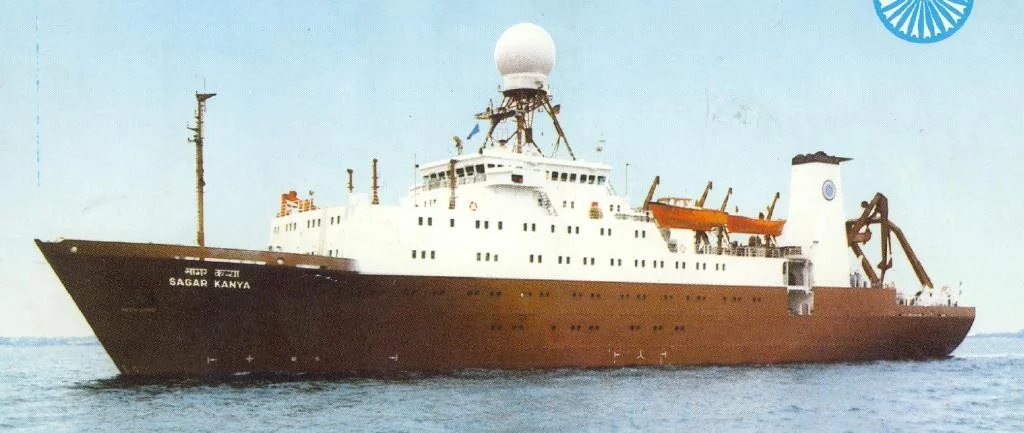
The research vessel Sagar Kanya at sea

Sagar Kanya · A. Jayaraman’s personal archive.

ATMOSPHERIC SCIENCE INDIAN OCEAN / DELHI / RANN

Discoveries
& expeditions.

Scientific expeditions change the vantage point: across an ocean, through a winter atmosphere, over a city and above a bright desert.

THE QUESTION

How does a field investigation become scientific evidence?

An ocean that carried the continent

The ocean surface can look remote from a city. The air above it can still carry a continental history.

During the Indian Ocean Experiment, ships, aircraft, satellites and ground stations investigated how aerosols crossed the region and altered radiation. Sagar Kanya supplied a moving laboratory: a way to sample changing air masses along a long ocean route rather than watch them from one fixed site.

The campaign chronology matters. A pre-INDOEX cruise ran from 5 January to 4 February 1996 and was reported in a 1998 paper led by A. Jayaraman. The later intensive phase included a Sagar Kanya cruise from 20 January to 12 March 1999. Jayaraman, Satheesh, Mitra and Ramanathan reported its latitude-dependent aerosol properties in Current Science in 2001. These are related investigations, separated by years. The 1996 study ↗ The 1999 cruise study ↗
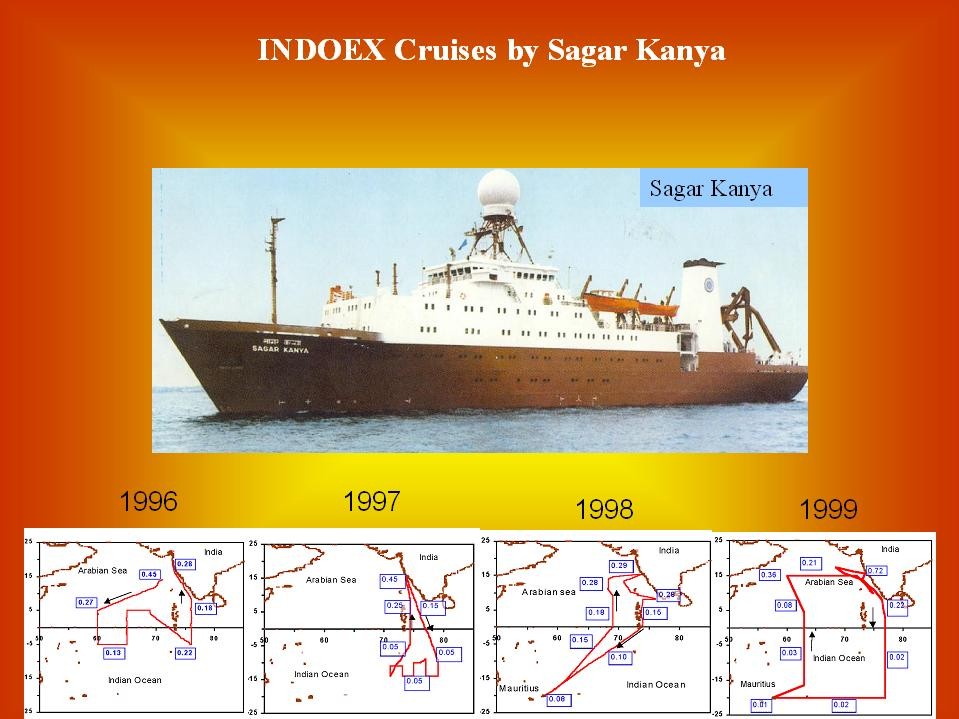
Sagar Kanya and the INDOEX cruise routes for 1996, 1997, 1998 and 1999
An observing programme built over successive cruisesSagar Kanya and the routes for 1996–1999 place the 1999 intensive campaign within the wider INDOEX sequence. Each route samples a different period as well as a changing region.A. Jayaraman’s personal archive.View image

The scientific question was not simply whether pollution existed offshore. It was how aerosol properties changed across contrasting air masses, including across the Inter Tropical Convergence Zone, and what those differences meant for radiation. A moving ship could connect a geographic gradient to several properties of the particles.

Sun photometry measured optical depth through the atmospheric column above the ship. Other instruments measured near-surface particle mass and size, scattering and absorption. These measurements were complementary. Deck-level air could differ from an elevated layer affecting the Sun’s beam, and particle water uptake could change scattering without a proportional change in dry mass.

The observations revealed a strong north–south contrast in aerosol properties across the sampled convergence region. Continental influence extended over the northern ocean, while the more southerly air masses differed. This was a meteorological and chemical transition, rather than a fixed latitude separating two permanent atmospheres.

Shipboard work introduced its own source problem: the ship. Measurements needed attention to wind direction and possible exhaust contamination. Instruments with different sampling and angular responses also required separate interpretation. A convincing gradient could not be established merely by plotting every reading in route order.

Radiation measurements and calculations connected aerosol properties to changes in sunlight. An absorbing component could reduce solar energy at the surface while adding energy within the atmosphere. The result helped make the Indian Ocean a setting for studying continental aerosol influence, rather than assuming a marine atmosphere was controlled only by sea spray.

How to read a cruise comparison

Check the sampling date as well as the latitude. A ship moves through weather that also evolves. Inspect exhaust screening, humidity treatment, spectral bands, instrument calibration and the relation between the near-surface and column samples. An apparent spatial pattern can include temporal variability.

The lasting contribution is methodological as well as geographical: a distant ocean can be understood by measuring several properties together and tracing the air’s changing context.

What kind of particle population crossed the sea?

The size distribution asks a more specific question than total loading. The comparison from the personal archive below sets an Arabian Sea size distribution against a maritime aerosol model and shows several fitted modes.
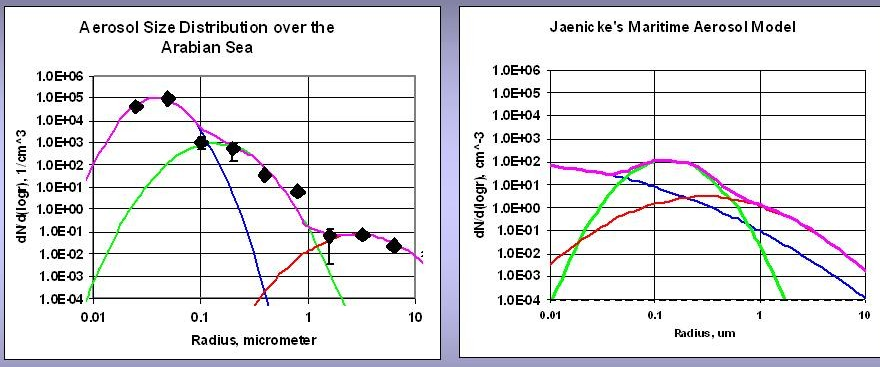
Arabian Sea aerosol size distribution and a maritime aerosol model
An oceanic atmosphere with a continental contributionRadius is in µm and dN/dlog r is in cm⁻³. Smooth curves represent fitted modes and the maritime model.A. Jayaraman’s personal archive.View image

The enhanced fine-particle part of the plotted distribution illustrates the contrast with the maritime model.

Ramanathan and colleagues’ integrated INDOEX analysis combined measurements from several platforms with models to connect aerosol composition and optical properties to radiative forcing and regional climate effects. The paper documented a mixture of inorganic and carbonaceous particles, including absorbing black carbon, rather than an atmosphere controlled only by sea spray. The integrated INDOEX analysis (2001) ↗
Fog has a vertical structure

A winter morning is seen from inside the atmosphere. That viewpoint hides how much changes with height.

In December 2004, Ganguly, Jayaraman, Rajesh and Gadhavi investigated aerosol properties during foggy and nonfoggy conditions over Delhi. They combined physical and optical measurements with vertical profiling to ask how the atmospheric state changed and what it meant for shortwave radiation. Read the study ↗

Three quantities must be kept distinct. Mass concentration reports sampled particle material per volume. Extinction is attenuation per distance. AOD integrates extinction vertically. Fog droplets and water-swollen particles affect light, while a dry aerosol measurement describes a different sampling condition.

The published profile comparison included 16 December, described as clear; 18 December, foggy; and 29 December, hazy. Those were observations on different days, with different meteorology. They were not three experimental settings imposed on an otherwise identical atmosphere.

A separate hourly sequence on 23 December followed the changing vertical structure from early morning into the afternoon. The authors interpreted the changes through redistribution and lifting within the lower atmosphere, with weak horizontal ventilation during the episode. The sequence concerned a particular day, rather than every Delhi winter.

Humidity and confinement supply two mechanisms for interpreting such observations. A shallow stable layer can concentrate particles near the surface. Hygroscopic growth increases their wet size and scattering. Daytime mixing can then redistribute extinction vertically. None of these mechanisms, by itself, identifies a changing emission rate.

The radiation analysis used aerosol observations to constrain a radiative-transfer model. It therefore estimated energy effects from measured properties and modelling assumptions; a photograph of fog was not the forcing measurement. The distinction between surface and top-of-atmosphere flux changes was essential to understanding atmospheric absorption.

Nearby Hisar supplied a separate study of clear, hazy and foggy conditions, led by Ramachandran and collaborators. It offers a comparison rather than a substitute dataset. Different sites, sampled episodes and methods must remain visible when results are compared. Read the study ↗

The Delhi campaign teaches a durable habit: before explaining a changing haze signal, locate it vertically, check humidity and identify where measurement ends and modelling begins.

When the lowest layer clears first

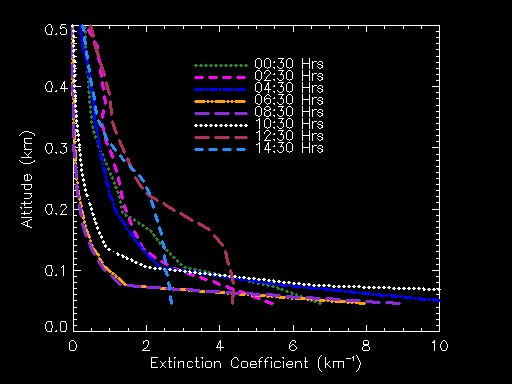
A mobile-lidar sequence from Delhi follows the vertical shape of extinction from 00:30 to 14:30. It makes a familiar visual impression more precise: improved visibility close to the ground can coexist with stronger extinction just above it.

Delhi aerosol extinction profiles from 00:30 to 14:30 across the lowest half-kilometre
A fog layer changing with height and timeExtinction coefficient in km⁻¹ is plotted against altitude over the lowest 0.5 km. The successive curves separate changes near the ground from those in the layer above.A. Jayaraman’s personal archive.View image

The lowest lidar ranges require particular care because transmitter–receiver overlap limits the retrieval. The structure above that range is the reason to measure vertically rather than rely only on a view from eye level.

The satellite and the bright salt desert

To measure a faint atmospheric contribution, first understand the bright surface beneath it.

A satellite looking at reflected sunlight receives a mixture of atmospheric scattering and surface reflection. An aerosol algorithm must separate them. The bright salt terrain of the Rann of Kuchchh makes that separation a particularly informative test.

A satellite receives light from both the surface and atmosphereSunSensorAtmospheric contributionSurface reflectionThe retrieval must separate these contributions.
Passive satellite observation, schematic. Surface brightness, aerosol assumptions, wavelength and viewing geometry all affect retrieval sensitivity.

Misra, Jayaraman and Ganguly examined historical MODIS retrieval performance over western India. Their 2015 paper assessed Collection 5.1 Dark Target and Deep Blue approaches using observations from 2002–2005. The version and period are part of the result: the study does not evaluate every later product. Read the study ↗

Dark Target was designed around assumptions suited to relatively dark land surfaces. Deep Blue uses spectral behaviour that supports retrieval over some brighter terrain. In the study, Deep Blue supplied retrievals over the bright Rann where Dark Target struggled to provide them.

Yet coverage and agreement were separate questions. More successful retrieval attempts over a surface did not mean stronger correlation with ground measurements everywhere. Overall Ahmedabad correlations in this historical comparison were stronger for Dark Target. Algorithm performance could not be reduced to a single winner.

Correlation alone also leaves bias and scatter unresolved. A retrieval can follow variability while remaining systematically high or low. Validation therefore needs matched overpass windows, quality screening and the uncertainty of the ground measurement as well as the satellite product.

An earlier 2008 study by the same authors compared MODIS collections against Microtops observations. Improved surface representation helped, while aerosol-model assumptions still affected results. Together, these investigations show retrieval development as a physical measurement problem, not simply a software version change. Read the study ↗

Research note: what a comparison must match

Inspect wavelength, pixel aggregation, ground-station representativeness, time difference, cloud screening and quality flags. A point measurement and a satellite pixel sample different spatial supports. Local variability can contribute to disagreement even when both instruments work as intended.

The wider lesson extends far beyond a salt desert. Every remote-sensing colour map rests on a forward model and an inverse problem. Validation asks where that chain is trustworthy and why it may fail.

Turn the lidar upside down

In February 2004, a compact micro-pulse lidar looked down from an aircraft over Hyderabad. Two sorties, on the evening of 17 February and the morning of 18 February, supplied a view of aerosol structure from above. Gadhavi and Jayaraman reported the study in 2006. Read the study ↗

The choice changed the observing geometry. Layers in the free troposphere could be examined from a different vantage point, and several extinction-retrieval algorithms could be compared. The return signal still depended on backscatter, attenuation and retrieval assumptions.

The investigators then tested radiative calculations with different vertical profiles while holding several column optical properties constant. The computed energy effect changed, demonstrating that an integrated AOD was not enough to specify the atmosphere’s radiative response.

This was not just a new view for its own sake. It connected an engineering decision—where to put the lidar and where to point it—to a scientific question about the vertical placement of aerosol.

CONNECTED READING

Inside the measurement ↗

Explore the aircraft, instrument geometry and lidar pulse experiment.

A small signal at Maitri

Low aerosol loading does not remove the need for careful radiation physics. At Maitri, India’s Antarctic station, measurements during 18 January–23 February 2001 combined sun photometry with near-surface aerosol mass and size observations. Gadhavi and Jayaraman reported the investigation in 2004. Read the study ↗

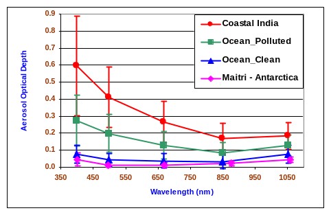
The study found low optical depth during the sampled polar summer, with a mean spectrum influenced by both fine and coarse material. Sampling was arranged away from the main station to reduce local contamination. Even in a remote environment, station activity and changing air masses had to be considered.

Antarctica supplied a useful contrast with the Indian Ocean. A bright surface reflects substantial light upward, and the seasonal solar geometry changes strongly. Radiative-transfer calculations showed how the energy effect could vary in magnitude and sign as illumination changed, even in an assumed constant-aerosol scenario.

That annual variation was a modelling sensitivity experiment, not a year-long aerosol observation. The distinction lets a short expedition answer a wider physical question without pretending it measured every season.

The case brings the chapters together: a low AOD is not a complete radiative description. Surface reflectance, particle optics and solar geometry determine what that small atmospheric signal means for energy.

Aerosol optical-depth spectra for coastal India, polluted ocean, clean ocean and Maitri
A spectrum from continental to polar conditionsThe labelled spectra compare coastal India, polluted-ocean and clean-ocean air with Maitri in Antarctica. Optical depth is dimensionless and wavelength is in nanometres. Both the magnitude and spectral shape differ across these sampled environments.A. Jayaraman’s personal archive.View image

A low aerosol signal makes calibration and molecular corrections especially consequential. The Maitri Langley measurement shows how the intensity reference is established before an aerosol optical depth can be interpreted.

A laboratory on the road

The same period also saw a mobile observatory carry complementary aerosol instruments through central India. The February 2004 road campaign, reported by Jayaraman and colleagues in 2006, combined vertical, column and near-surface measurements. Read the study ↗

Its strength was the ability to examine changing aerosol characteristics across a regional route. Its interpretive challenge was that route position, date and weather changed together. A difference between two stops was not automatically a difference in local emissions.

Ocean, road and airborne experiments share that discipline. They enlarge the observing domain, then require careful matching of what each instrument sampled. The resulting papers are strongest when they carry the geometry, timing and assumptions into the scientific conclusion.

CONNECTED READING

The people behind the measurements ↗

Follow the collaborations and instrument lineage across these investigations.

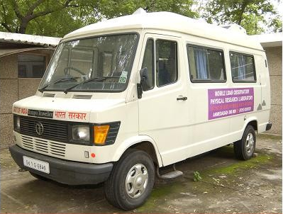
The PRL mobile atmospheric laboratory
Carry the vertical view along the roadThe PRL mobile laboratory made the lidar and its supporting electronics part of a travelling observing platform. A route extends the range of places sampled, while time and meteorology continue to change.A. Jayaraman’s personal archive.View image
PAPERS & FURTHER READING

Follow the
evidence.

  1. A. Jayaraman, D. Lubin, S. Ramachandran, V. Ramanathan, E. Woodbridge, W. D. Collins & K. S. Zalpuri (1998). Direct observations of aerosol radiative forcing over the tropical Indian Ocean during the January–February 1996 pre-INDOEX cruise. Journal of Geophysical Research 103, 13827–13836 ↗
  2. A. Jayaraman, S. K. Satheesh, A. P. Mitra & V. Ramanathan (2001). Latitude gradient in aerosol properties across the Inter Tropical Convergence Zone: Results from the joint Indo-US study onboard Sagar Kanya. Current Science 80, supplement, 128–137 ↗
  3. V. Ramanathan et al., including A. Jayaraman (2001). Indian Ocean Experiment: An integrated analysis of the climate forcing and effects of the great Indo-Asian haze. Journal of Geophysical Research: Atmospheres, 106(D22), 28371–28398. DOI: 10.1029/2001JD900133 ↗
  4. H. Gadhavi & A. Jayaraman (2004). Aerosol characteristics and aerosol radiative forcing over Maitri, Antarctica. Current Science 86(2), 296–304 ↗
  5. A. Jayaraman, H. Gadhavi, D. Ganguly, A. Misra, S. Ramachandran & T. A. Rajesh (2006). Spatial variations in aerosol characteristics and regional radiative forcing over India: measurements and modeling of 2004 road campaign experiment. Atmospheric Environment ↗
  6. D. Ganguly, A. Jayaraman, T. A. Rajesh & H. Gadhavi (2006). Wintertime aerosol properties during foggy and nonfoggy days over urban center Delhi and their implications for shortwave radiative forcing. Journal of Geophysical Research 111, D15217 ↗
  7. H. Gadhavi & A. Jayaraman (2006). Airborne lidar study of the vertical distribution of aerosols over Hyderabad, an urban site in central India, and its implication for radiative forcing calculations. Annales Geophysicae 24, 2461–2470 ↗
  8. S. Ramachandran, R. Rengarajan, A. Jayaraman, M. M. Sarin & S. K. Das (2006). Aerosol radiative forcing during clear, hazy, and foggy conditions over a continental polluted location in north India. Journal of Geophysical Research 111, D20214 ↗
  9. A. Misra, A. Jayaraman & D. Ganguly (2008). Validation of MODIS derived aerosol optical depth over Western India. Journal of Geophysical Research 113, D04203 ↗
  10. A. Misra, A. Jayaraman & D. Ganguly (2015). Validation of Version 5.1 MODIS Aerosol Optical Depth (Deep Blue Algorithm and Dark Target Approach) over a Semi-Arid Location in Western India. Aerosol and Air Quality Research 15, 252–262 ↗
  11. A. Jayaraman · Personal archive. Atmospheric research photographs, instrument diagrams and observations. Personal archive ↗

Image

100%Open image ↗