A photometer detects light. A lidar records returned photons. A particle counter registers an instrument response. The atmospheric quantity comes next.
Observation starts with a physical signal, calibration and a sampling geometry. Analysis then separates atmospheric contributions and uses a model to infer a quantity such as optical depth, extinction or particle size. Each step introduces assumptions and uncertainty.
This chain is not a weakness to hide. It is what makes a result testable. Another instrument can constrain a different part of the chain, while a known calibration target can reveal drift. Metadata such as wavelength, time, height and averaging interval are part of the measurement.
A sun photometer measures direct solar intensity through narrow spectral bands. A reduction from the calibrated extraterrestrial intensity contains information about extinction along the path. Molecular scattering and gas absorption must be accounted for before assigning the remaining attenuation to aerosol.
Calibration determines the reference signal; cloud screening prevents cloud attenuation from being misread as aerosol. Pointing, spectral response and the Sun’s elevation also matter. The output AOD is a column property at a specified wavelength, not a surface particle mass.
A 1995 instrument paper by Acharya, Jayaraman, Ramachandran and Subbaraya used an LED as a spectrally selective detector and as a nonlinear feedback element. The logarithmic electronic response connected intensity attenuation with optical depth. The ingenuity lay in the whole measurement system, including response and calibration. The paper acknowledged earlier LED detector work. Read the study ↗
Methods: the slope and the intercept
Taking logarithms of Beer–Lambert attenuation gives ln I = ln I₀ − mτ for a stable column after appropriate corrections. A Langley analysis relates log signal to air mass to estimate an intercept. Changes in the atmosphere during calibration, or an incorrect gas correction, can bias the inferred aerosol optical depth.
Keep the Sun in view
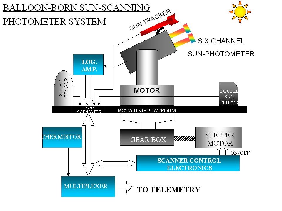
The balloon instrument developed at PRL combined Sun tracking with a rotating scanning platform. Its channels observed direct and scattered radiation while the electronics linked the optical signals to telemetry.
Tracking and scanning from a balloonThe sun tracker, multi-channel photometer, motor-driven platform and telemetry form one observing system. Stable pointing and known spectral response are essential to interpreting the light.A. Jayaraman’s personal archive.View image ↗
A calibration in the Antarctic sky
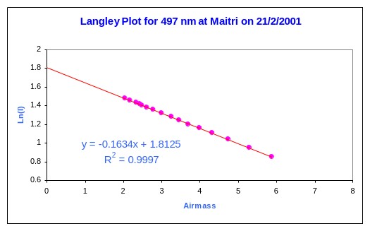
At Maitri on 21 February 2001, measurements at 497 nm followed the Sun as its atmospheric path length changed. Plotting the logarithm of intensity against relative airmass produced a nearly straight line.
A Langley measurement at MaitriThe fitted slope has magnitude 0.1634 and describes total atmospheric optical depth at 497 nm for this measurement. Molecular scattering and gas absorption must be accounted for to obtain the aerosol contribution. The intercept estimates the signal at zero airmass.A. Jayaraman’s personal archive.View image ↗
This is the practical role of calibration: establish a reference for the instrument, then separate the atmospheric contributions. A close fit alone does not make the slope an aerosol-only measurement. Read the study ↗
Lidar emits a pulse and measures light scattered back towards the receiver. The delay supplies range. The return strength depends on how much light is scattered towards the instrument, how much is attenuated on the outward and return paths, and the instrument’s geometry and response.
Elastic backscatter lidar therefore faces an inverse problem: both extinction and backscatter affect one return signal. Retrieving extinction commonly requires an assumed relationship between them and a reference condition. Raman and high-spectral-resolution methods supply additional information that can reduce this ambiguity.
Near the instrument, transmitter and receiver fields may not fully overlap. Dense cloud or aerosol can attenuate the beam so strongly that little useful information returns from beyond it. A weak return is not always an empty atmosphere.
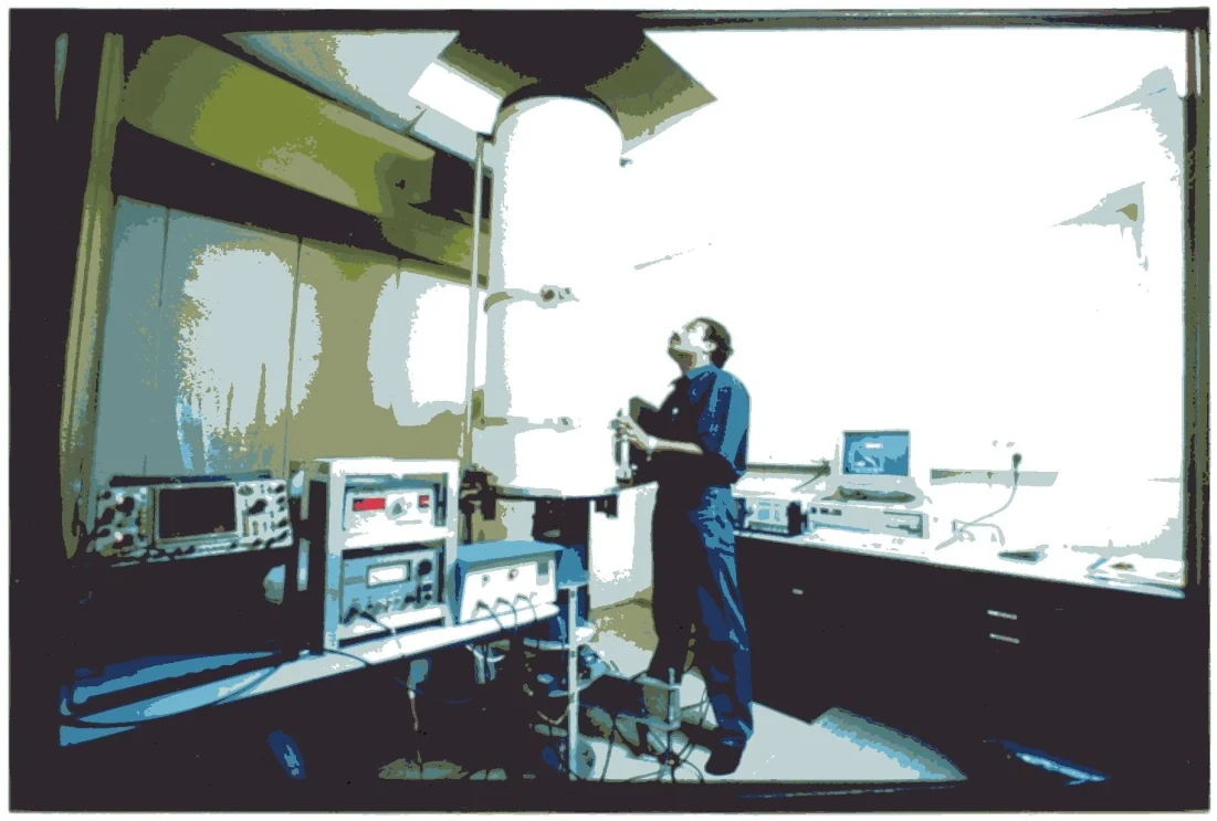
An early Indian backscatter lidarThe Nd:YAG backscatter lidar developed at PRL, Ahmedabad, in 1991. This archival view records the instrument and its working setting; it is a different system from the compact micro-pulse lidar shown below.A. Jayaraman’s personal archive.View image ↗
EXPERIMENT / TIME OF FLIGHT
Send a pulse. Measure the distance.
A laser pulse must travel to the layer and back. Choose a range and read the return time.
Physics and assumptions
R = cΔt / 2, using c ≈ 299,792,458 m s⁻¹. Range is distance from the instrument along the beam. It equals height above the instrument only for a vertical beam.
Pulse width, detector timing and averaging limit range resolution. Return strength also depends on backscatter, attenuation, geometric spreading and instrument overlap; time alone gives no aerosol mass.
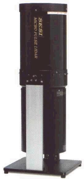
Inside the micro-pulse lidar
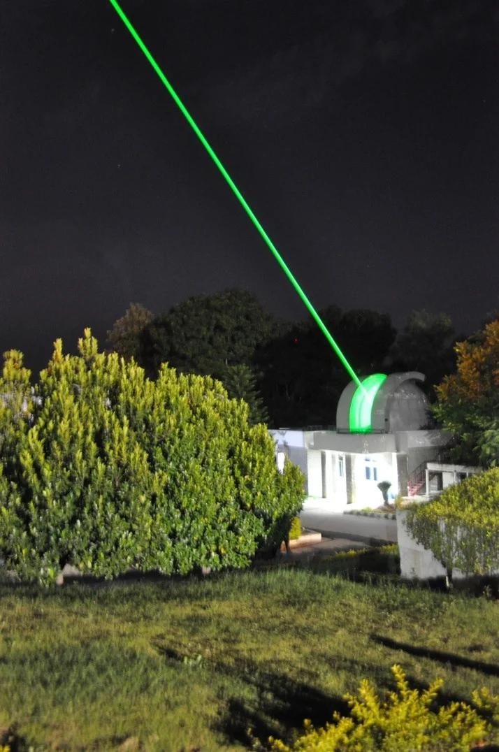
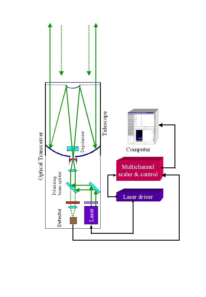
A compact housing contains a transmitter, a receiver telescope and photon-counting detection. The optical arrangement must keep the outgoing pulse and the returning signal distinguishable while their fields of view overlap in the atmosphere.
A compact observing instrumentThe micro-pulse lidar brings the transmitter and receiver into a small instrument that can be used from several platforms.A. Jayaraman’s personal archive.View image ↗Trace the optical returnThe original schematic connects the laser, beam expander, telescope, detector and data system. It shows why the signal depends on the receiving optics as well as the transmitted pulse.A. Jayaraman’s personal archive.View image ↗
A balloon can carry instruments through atmospheric layers. Optical payloads measure radiation from within a changing geometry; particle counters sample air around the payload, subject to their size response. A flight yields a detailed profile along a moving path, not a continuous daily record at one fixed column.
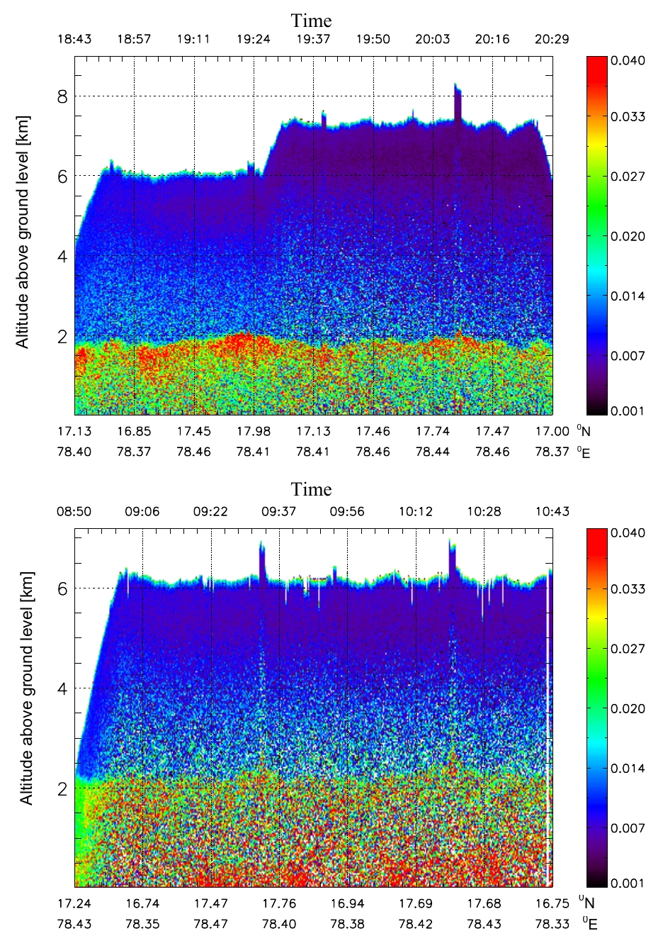
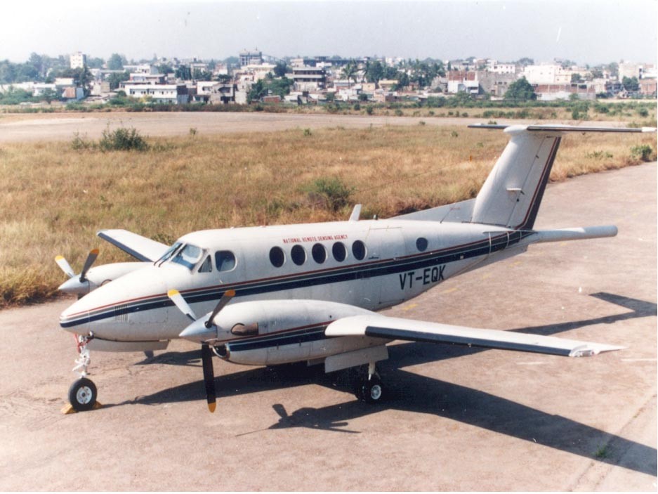
An aircraft can map structure along tracks and revisit a region. Over Hyderabad on 17 and 18 February 2004, a compact micro-pulse lidar was installed looking downward in a Beech Superking aircraft. Gadhavi and Jayaraman compared extinction retrieval methods and used the observed structure in radiative-transfer calculations. Read the study ↗
The downward view supplied a different perspective on the free troposphere from the same lidar used on the ground. Geometry changed which layers were easiest to examine; it did not eliminate retrieval assumptions. The aircraft result is a concrete demonstration of why platform design belongs in scientific interpretation.
Gadhavi & Jayaraman (2006). Normalised relative backscatter in arbitrary units, with altitude above ground in km. Upper panel: 17 February; lower: 18 February. Colour represents the optical return, not aerosol mass. Original paper · CC BY 3.0. Open full resolution ↗
Read height vertically and measurement sequence horizontally. The authors identified a boundary-layer top near 2 km on both days, while the structure within the layer differed. The changing upper boundary of each curtain also reflects the aircraft’s viewing geometry; blank space is not evidence of particle-free air.
A platform above the aerosol layerAircraft VT-EQK carried the downward-looking micro-pulse lidar used over Hyderabad on 17–18 February 2004. The geometry and analysis are reported by Gadhavi & Jayaraman (2006).A. Jayaraman’s personal archive.View image ↗
A passive satellite sensor receives radiance containing contributions from the atmosphere and the surface. An aerosol retrieval compares that signal with calculations that assume surface reflectance, particle properties and viewing geometry. A bright surface can make the atmospheric contribution especially difficult to isolate.
Different algorithms exploit different wavelength and surface behaviour. Historical MODIS validation over western India compared retrievals with ground photometry and examined the bright Rann of Kuchchh. The study exposed a distinction between retrieving more scenes and retrieving accurate values in those scenes. Read the study ↗
Passive satellite observation, schematic. Surface brightness, aerosol assumptions, wavelength and viewing geometry all affect retrieval sensitivity.
Satellite lidar adds vertical information along a narrow track. Comparing it with a ground lidar requires compatible timing, height, wavelength and cloud screening. The Gadanki cirrus work used these complementary views rather than treating the satellite as an unquestionable reference. Read the study ↗
A nephelometer measures scattering in sampled air over its instrument’s angular response. An absorption photometer measures an absorption-related signal that may need corrections for its filter or optical method. A radiometer measures radiant flux or radiance over its spectral and angular response. A mass instrument and an optical instrument are not measuring interchangeable quantities.
Humidity conventions can matter as much as location. An inlet may dry sampled particles while an atmospheric optical measurement sees them wet. Averaging over an hour, a day or a satellite overpass changes which variability remains visible.
For a useful comparison, match the property, wavelength, sample volume, humidity treatment and time window. Then inspect calibration, uncertainty and retrieval assumptions. Agreement is more convincing when the methods have genuinely independent strengths and limitations.